Analysis of Bayesian Model Misspecification

Comparing Bayesian predictive distributions under examples of model misspecification.

Introduction

Bayesian methods combine prior beliefs with observed data to update uncertainty, but they are still vulnerable to model misspecification, where assumed structure (like independence or hierarchy) does not match the true data-generating process.

This project asks: if two models have nearly the same prior predictive behavior, how much can mild structural misspecification still change posterior predictions?

We test two cases:

1. Data are hierarchical, but the analysis model is flat.
2. Data are dependent, but the analysis model assumes independence.

In both cases, posterior predictive distributions diverge meaningfully after seeing the same data. The practical takeaway is that a model can look well calibrated before observing data and still give misleading posterior inferences if its structure is wrong.

Example 1. Real data is hierarchical, but assumed to be flat.

Our data \(y\) follows the following hierarchical distribution, which we’ll denote \(D_1\).

\[ \begin{align} Y &\sim Binom(100, p) \\ p &\sim Beta(3, 4) \end{align} \]

n_obs = 100
y = r_beta_bernoulli(n_obs, alpha = 3, 4)
y_obs = sum(y)
y_obs

[1] 42

Now, we will misspecify the model.

We now assume the data comes from a binomial distribution, and assign a beta(5,3) prior on the proportion, where Y is the sum of the data, We’ll call this model \(M\) (for “Misspecified”). \[ \begin{aligned} Y &\sim \text{Binom}(n = 100, p) \\ (Prior)\quad p &\sim \text{Beta}(5, 3) \end{aligned} \]

Prior Predictive distribution:

pp_sample_size = 10000

# the predictive distribution follows a beta-binomial
prior_pred_M = r_beta_binom(pp_sample_size, n_obs, 5, 3)

Now to find an equivalent prior for the real model

The real model (\(D_1\)): \[ \begin{aligned} Y &\sim \text{Binom}(n=100, p) \\ p &\sim \text{Beta}(\alpha, \beta) \\ (Prior)\quad \alpha &\sim \log \mathcal{N}(\mu_1, \sigma_1) \\ (Prior)\quad \beta &\sim \log \mathcal{N}(\mu_2, \sigma_2) \end{aligned} \]

A function to sample from the prior predictive distribution:

# function for sampling from prior predictive distrib of D2 model
sample_from_pp_D1 = function(n, size, mu1, sigma1, mu2, sigma2) {
  alphas = rlnorm(n, mu1, sigma1)
  betas = rlnorm(n, mu2, sigma2)
  probs = rbeta(n, alphas, betas)
  sample = rbinom(n, size, probs)
  return(sample)
}

We will use lognormal \(\log \mathcal{N}(\log 5,\ 0.01)\) and \(\log \mathcal{N}(\log 3,\ 0.01)\) as the priors for \(\alpha\) and \(\beta\) in model \(D_1\), chosen to create a very similar prior predictive distribution to the prior for \(M\).

These are the prior predictive distributions compared:

prior_pred_D1 = sample_from_pp_D1(n = pp_sample_size,
                                 size = n_obs,
                                 mu1 = log(5), sigma1 = 0.01,
                                 mu2 = log(3), sigma2 = 0.01)

tvd_prior = pp_sample_distance(prior_pred_D1, prior_pred_M)
tvd_prior

[1] 0.0447

plot_pp_difference(real_sample = prior_pred_D1, real_model_name = "D1",
                   miss_sample = prior_pred_M, miss_model_name = "M",
                   prior_or_post = "Prior")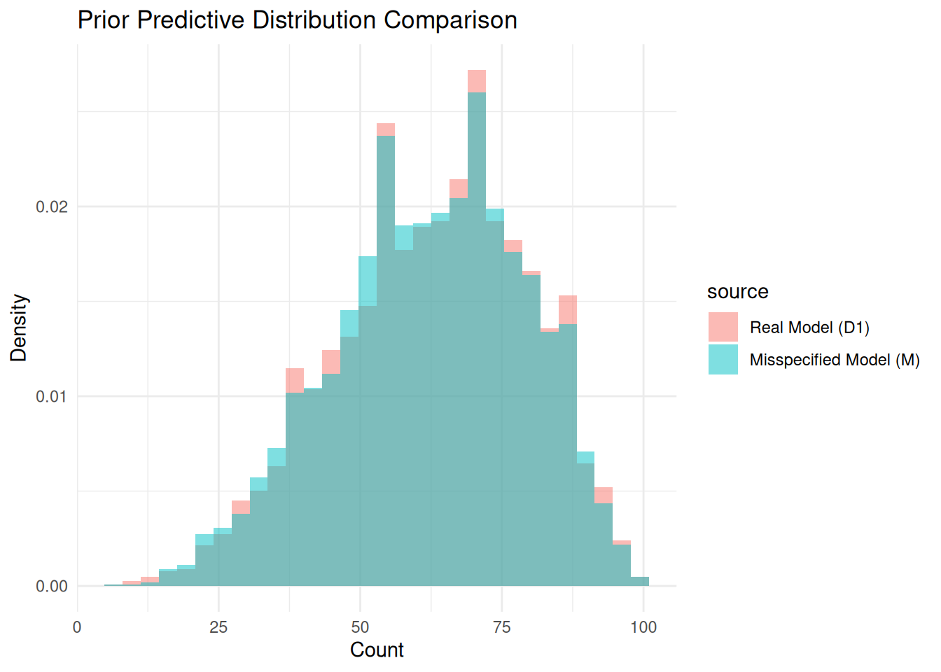

As shown, the prior predictive distributions are extremely similar, so these priors are effectively equivalent.

That means any posterior differences after updating on data should mostly come from model structure, not prior choice.

Now we update both models and compare the posterior predictives.

Updating \(D_1\)

We approximate the posterior with naive simulation (rejection sampling).

# We sample from the prior a lot, predict with the param values from the prior,
# and keep if the prediction is equal to the observed data

df = data.frame(alpha = numeric(), beta = numeric())

i = 1
while (i <= pp_sample_size) {
  alpha = rlnorm(1, log(5), 0.01)
  beta = rlnorm(1, log(3), 0.01)
  
  y_pred = r_beta_binom(1, n_obs, alpha, beta)
  
  if (y_pred == y_obs) {
    df = rbind(df, data.frame(alpha=alpha, beta=beta))
    i = i+1
  }
}

df <- mutate(df, post_pred = r_beta_binom(n(), n_obs, alpha, beta))

Updating \(M\)

This is a straightforward application of the Beta-Binomial Prior.

\[ Y \sim Binom(100, p), \quad p \sim Beta(5, 3) \]

so \[ p \mid Y = 42 \sim Beta\!\big(5+42,\ 3+58\big) \]

post_predictive_M = r_beta_binom(pp_sample_size, n_obs, 5+y_obs, 3+n_obs-y_obs)

Comparing analysis for \(M\) vs equivalent analysis for \(D_1\)

tvd_post = pp_sample_distance(df$post_pred, post_predictive_M)

plot_pp_difference(real_sample = df$post_pred, real_model_name = "D1",
                   miss_sample = post_predictive_M, miss_model_name = "M",
                   prior_or_post = "Posterior")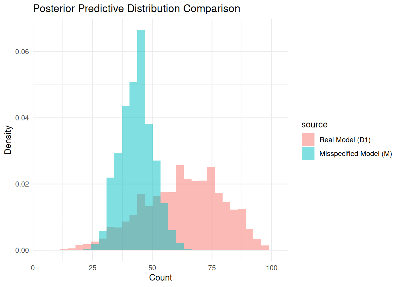

The posterior predictives are clearly different, with total variation distance 0.648 (a 14.4966443-fold increase over prior TVD). In this setup, misspecification has a meaningful effect on inference.

Example 2. Real data is dependent, but assumed to be independent.

Now we test a dependence misspecification case. Data are generated by summing a Markov process of \(n\) drifting Bernoulli trials (model \(D_2\)).

\[ Y \sim MC(n=100, \ p_0=0.4, \ \delta=0.1) \] (MC = Markov Counts; sampling details are in helper functions.)

Here, \(p_0\) is the initial success probability and \(\delta\) is the standard deviation of Gaussian drift added to the success probability after each trial.

n_ops = 100
y = r_markov_bernoulli(n_ops, p0=0.4, drift_sd=0.1)
y_obs = sum(y)
y_obs

[1] 34

Again, we intentionally misspecify by fitting a binomial model with the same \(\text{Beta}(5, 3)\) prior on \(p\) (model \(M\)). \[ \begin{aligned} Y &\sim \text{Binom}(n=100, p) \\ (Prior)\quad p &\sim \text{Beta}(5, 3) \end{aligned} \]

Now we choose an equivalent prior for model \(D_2\). \[ \begin{aligned} Y &\sim MC(n=100, p_0, \delta) \\ (Prior)\quad p_0 &\sim \text{Beta}(\alpha, \beta) \\ (Prior)\quad \delta &\sim \text{Exp}(\lambda) \end{aligned} \] We use the function below to sample from the prior predictive distribution of \(D_2\).

sample_from_pp_D2 = function(n, size, alpha, beta, rate) {
    p0 = rbeta(n, alpha, beta)
    drift_sd = rexp(n, rate)
    sample = r_markov_counts(n, size, p0, drift_sd)
    return(sample)
}

We use this prior distribution: \[ \begin{aligned} Y &\sim MC(n=100, \ p_0, \ \delta) \\ (Prior)\quad p_0 &\sim \text{Beta}(5, 3) \\ (Prior)\quad \delta &\sim \text{Exp}(100) \end{aligned} \]

Now compare the prior predictive distributions:

prior_pred_D2 = sample_from_pp_D2(n=pp_sample_size,
                                  size = n_obs,
                                  alpha=5, beta=3, rate=100)

tvd_prior = pp_sample_distance(prior_pred_D2, prior_pred_M)
tvd_prior

[1] 0.0601

plot_pp_difference(real_sample = prior_pred_D2, real_model_name="D2",
                   miss_sample = prior_pred_M, miss_model_name="M",
                   prior_or_post = "Prior")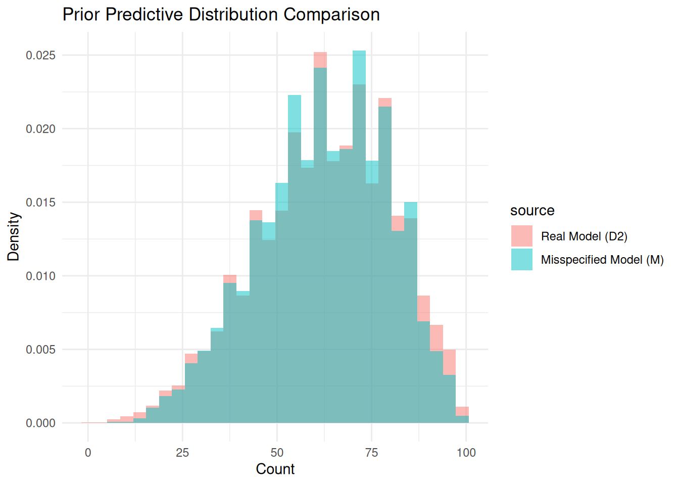

Again, the prior predictives are effectively equivalent.

Next we update both models and measure how much the posterior predictives diverge.

Updating \(D_2\)

We use naive simulation again to get a posterior sample for \(D_2\).
This step is slower, so we accept draws within 1 of the observed count, which makes the approximation slightly rougher.

df = data.frame(p0 = numeric(), drift_sd = numeric())

i = 1
while (i <= pp_sample_size) {
  p0 = rbeta(1, 5, 3)
  drift_sd = rexp(1, 100)
  
  y_pred = r_markov_counts(1, n_obs, p0, drift_sd)
  
  if (abs(y_pred - y_obs) <= 1) {
    df = rbind(df, data.frame(p0=p0, drift_sd=drift_sd))
    i = i+1
  }
}

df <- mutate(df, post_pred = r_markov_counts(n(), n_obs, p0, drift_sd))

Updating \(M\)

Again, this is a straightforward Beta-Binomial update.

post_predictive_M = r_beta_binom(pp_sample_size, n_obs, 5+y_obs, 3+n_obs-y_obs)

Comparing Posterior Predictive Distributions:

tvd_post = pp_sample_distance(df$post_pred, post_predictive_M, method = 'tvd')

plot_pp_difference(real_sample = df$post_pred, real_model_name = "D2",
                   miss_sample = post_predictive_M, miss_model_name = "M",
                   prior_or_post = "Posterior")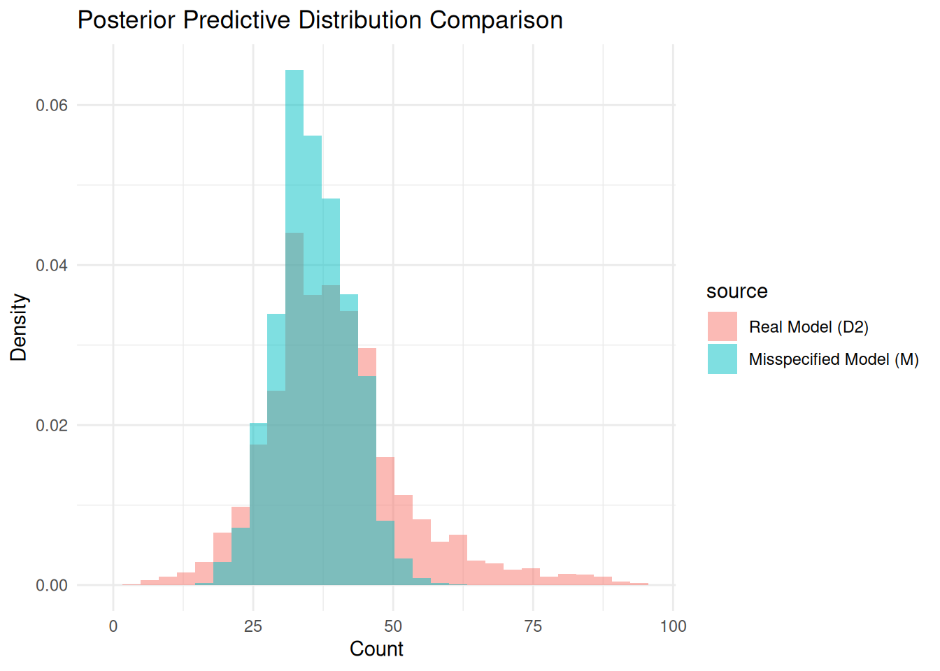

The total variation distance is 0.214 (a 3.5607321-fold increase from prior TVD), and the posterior predictive distributions are visibly different.

Conclusion

These examples show that mild misspecification can materially change Bayesian conclusions, even when prior predictive checks look reasonable. In practice, this is a warning: prior calibration is helpful, but it does not protect you if structural assumptions are wrong.

Future Work

A next step is to identify which analyses and test statistics stay robust under different kinds and degrees of misspecification. To do that, we need:

• A principled way to quantify how far a proposed model is from the true data-generating process.
• An efficient method for choosing priors on the true model that match the proposed model’s prior predictive distribution, so structural effects can be isolated cleanly. (2)

2. In practice, matching a target prior predictive distribution is hard because the prior search space is large. A more general and computationally efficient search method would make this workflow much more usable.

Appendix

Helper Functions

Functions are sourced at the top so they stay out of the way while reading. Full helper code is shown here for reference.

 r_beta_bernoulli = function(n, alpha, beta) {
  probs = rbeta(n, alpha, beta)
  sample = rbinom(n, 1, probs)
  return(sample)
}

r_beta_binom = function(n, size, alpha, beta) {
  probs = rbeta(n, alpha, beta)
  sample = rbinom(n, size, probs)
  return(sample)
}

r_markov_bernoulli = function(n, p0, drift_sd) {
  probs = numeric(n)
  probs[1] = p0
  
  for (i in 2:n) {
    probs[i] = probs[i - 1] + rnorm(1, 0, drift_sd)
    probs[i] = min(max(probs[i], 0), 1)
  }
  sample = rbinom(n, 1, probs)
  return(sample)
}

r_markov_counts = function(n, size, p0, drift_sd) {
  sample = numeric(n)
  for (i in 1:n) {
    sample[i] = sum(r_markov_bernoulli(size, p0[i], drift_sd[i]))
  }
  return(sample)
}

pp_sample_distance = function(pp_sample1, pp_sample2, method = "tvd") {
  
  if (length(pp_sample1) != length(pp_sample2)) {
    print("warning: sample sizes are different")
  }
  
  if (method == "tvd") {
    max_val = max(c(pp_sample1, pp_sample2))
    
    counts1 = tabulate(pp_sample1, nbins = max_val)
    counts2 = tabulate(pp_sample2, nbins = max_val)
    
    counts1 = counts1 / sum(counts1)
    counts2 = counts2 / sum(counts2)
    
    return(0.5 * sum(abs(counts1 - counts2)))
  } else if (method == "binned_tvd") {
    combined = c(pp_sample1, pp_sample2)
    breaks = hist(combined, plot = FALSE)$breaks
  
    counts1 = hist(pp_sample1, breaks = breaks, plot = FALSE)$counts
    counts2 = hist(pp_sample2, breaks = breaks, plot = FALSE)$counts
    
    counts1 = counts1 / sum(counts1)
    counts2 = counts2 / sum(counts2)
    
    return(0.5 * sum(abs(counts1 - counts2)))
  } else {
    print("available methods are 'tvd' and 'binned_tcd'")
  }
}

plot_pp_difference = function(real_sample, miss_sample, prior_or_post, real_model_name, miss_model_name) {
  
  plot_df = tibble(
   D = real_sample,
   M = miss_sample
  ) |> 
  pivot_longer(
    cols = D:M,
    names_to = "source",
    values_to = "values"
  )

  ggplot(plot_df, aes(x = values, fill = source)) +
    geom_histogram(aes(y = after_stat(density)), position = "identity", alpha = 0.5, bins = 30) +
    labs(title = glue("{prior_or_post} Predictive Distribution Comparison"), x = "Count", y = "Density") +
    scale_fill_discrete(
      labels = c(glue("Real Model ({real_model_name})"), glue("Misspecified Model ({miss_model_name})"))) + 
    theme_minimal()
}

sample_from_pp_D1 = function(n, size, mu1, sigma1, mu2, sigma2) {
  alphas = rlnorm(n, mu1, sigma1)
  betas = rlnorm(n, mu2, sigma2)
  probs = rbeta(n, alphas, betas)
  sample = rbinom(n, size, probs)
  return(sample)
}

sample_from_pp_D2 = function(n, size, alpha, beta, rate) {
    p0 = rbeta(n, alpha, beta)
    drift_sd = rexp(n, rate)
    sample = r_markov_counts(n, size, p0, drift_sd)
    return(sample)
}

r_markov_bernoulli_old = function(n, p_initial, p_after_1, p_after_0){
  sample = numeric(n)
  sample[1] = rbinom(1, 1, p_initial)
  for (i in 2:n) {
    if (sample[i - 1] == 1) {sample[i] = rbinom(1, 1, p_after_1)}
    else {sample[i] = rbinom(1, 1, p_after_0)}
  }
  return(sample)
}

r_markov_counts_old = function(n, size, p_initial, p_after_1, p_after_0) {
  sample = numeric(n)
  for (i in 1:n) {
    sample[i] = sum(r_markov_bernoulli_old(size, p_initial, p_after_1, p_after_0))
  }
  return(sample)
} 

Errata

We first tried grid search over parameterized priors to match prior predictives, but it performed poorly.

# grid = expand.grid(
#   mu1 = seq(1, 50, by=5),
#   mu2 = seq(1, 50, by=5),
#   sigma1 = seq(1, 50, by=5),
#   sigma2 = seq(1, 50, by=5)
# )

# grid = grid |> 
#   mutate(
#     pp_sample = pmap(
#       list(mu1, sigma1, mu2, sigma2),
#       ~ sample_from_pp_D1(n = pp_sample_size,
#                           size = n_obs,
#                           mu1 = ..1, sigma1 = ..2,
#                           mu2 = ..3, sigma2 = ..4))) |> 
#   mutate(
#     distances = map(pp_sample, ~ pp_sample_distance(.x, prior_pred_M))
#   ) |> 
#   arrange(distances)

We also tried a different Markov model variant, but could not find priors that produced equivalent prior predictives.

# (UNUSED because couldn't find equivalent predictive prior) function to sample Markov Bernoulli Distribution
r_markov_bernoulli_old = function(n, p_initial, p_after_1, p_after_0){
  sample = numeric(n)
  sample[1] = rbinom(1,1,p_initial)
  for (i in 2:n) {
    if (sample[i-1]==1) {sample[i] = rbinom(1,1, p_after_1)}
    else {sample[i] = rbinom(1,1, p_after_0)}
  }
  return(sample)
}

# (UNUSED because couldn't find equivalent predictive prior) function to sample counts from 'size'-number of markov bernoulli trials
r_markov_counts_old = function(n, size, p_initial, p_after_1, p_after_0) {
  sample = numeric(n)
  for (i in 1:n){ # for each sample, do 'size' bernoulli trials, then sum
    sample[i] = sum(r_markov_bernoulli(size, p_initial, p_after_1, p_after_0))
  }
  return(sample)
}